
Computational Geometry for Computer Vision
The field of computational geometry emerged in the 1970s and deals with the study of data structures and algorithms for solving geometric…


The field of computational geometry emerged in the 1970s and deals with the study of data structures and algorithms for solving geometric problems. This includes, in particular, the determination of topological structures within images, or indeed higher-dimensional representations, such as point neighbourhoods, which can help derive geometric meaning from, for example, digital image data [1].
Computer vision is primarily concerned with still or moving image processing, understanding and reconstruction [3]. Due to impressive, super-human results delivered by deep neural network-powered algorithms, the computer vision application areas of object identification (classification), object detection (classification & localisation) and object segmentation (classification, localisation & boundary detection) have been receiving steadily increasing attention in research and industry.
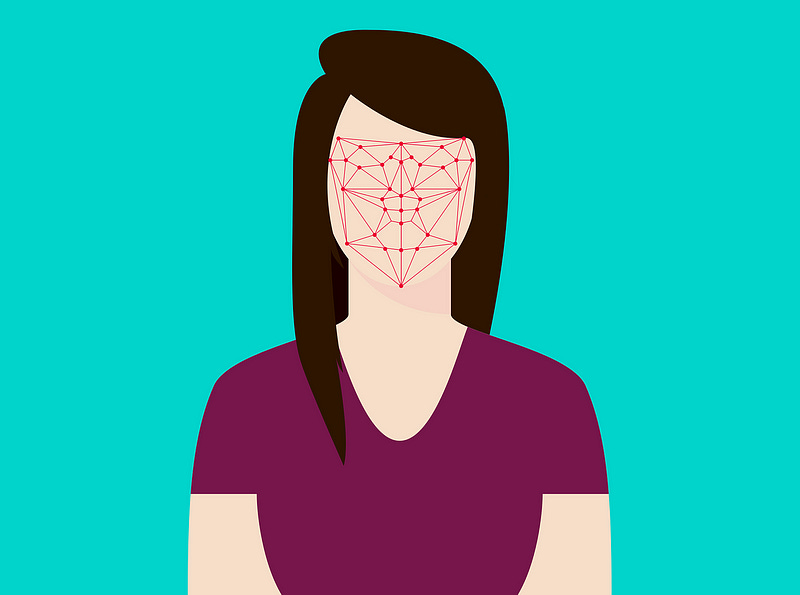
Unsurprisingly, given these overlapping areas of interest, computational geometry has useful concepts to offer to the field of computer vision, and its counterpart, computer graphics. The Voronoi diagram (a.k.a. Dirichlet tessellation, Voronoi tessellation or Voronoi partition) of a set of points, and its dual, the points’ Delaunay triangulation (a.k.a. Delone triangulation), are examples for such useful concepts [1, 2]. Relevant computer vision applications include face recognition, face morphing, image synthesis and surface modeling. In this blog post, we demonstrate the use of the Delaunay triangulation/Voronoi diagram of faces in images as a precursor for applications such as face recognition or face morphing.
Let’s start with definitions.
A Voronoi diagram partitions a domain into regions of closest neighbourhoods for a set of points. Consider the set of points P = {p₁, p₂, …, pₙ} ∈ ℝ². Define the bisector BS(pᵢ, pⱼ) of pᵢ, pⱼ ∈ P, pᵢ ≠ pⱼ, as equidistant loci with respect to pᵢ, pⱼ in the distance function d, i.e. BS(pᵢ,pⱼ) = {q ∈ P : d(pᵢ,q) = d(pⱼ,q)}. Let the dominance region of pᵢ with respect to pⱼ, D(pᵢ,pⱼ), denote the region containing pᵢ bounded by BS(pᵢ,pⱼ). The Voronoi region of pᵢ given P is defined as

and consists of all points for which the distance to pᵢ is smaller than or equal to the distance to any other point pⱼ ∈ P. The boundary shared by a pair of Voronoi regions is called a Voronoi edge. Voronoi edges meet at Voronoi vertices. The Voronoi diagram of P is given by

where ∂R(pᵢ,P) denotes the boundary of R(pᵢ,P). The term bounded Voronoi diagram refers to the conjunction of VD(P) with its underlying domain.
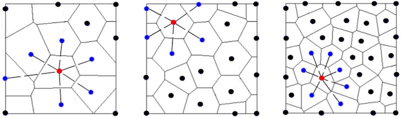
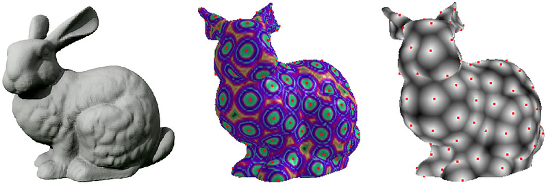
We restricted ourselves to points in the Euclidean planar domain, see, for example, Figure 1. The Voronoi diagram definition can, however, be generalised to points P acquired without noise from a manifold M, i.e. the more general case of P ⊂ M. See, for example, Figure 2 for an intrinsic (non-Euclidean) Voronoi diagram of points on a 3D manifold.
Similarly, we did not define a distance metric with respect to the distance function d: The Voronoi diagram definition holds for any geodesic distance metric defined across the manifold M. So, for example, in the Euclidean planar domain case, the standard Euclidean distance function can be used for the computation of d(⋅,⋅).
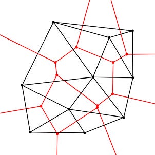
The Delaunay triangulation of the point set P = {p₁, p₂, …, pₙ} ∈ ℝ² is given by the dual graph of VD(P), with each edge of the Delaunay triangulation being associated with one edge of VD(P), i.e. the Delaunay edges connect (natural) neighbouring points in VD(P). See Figure 3 for an example. Delaunay triangulations generally exist for metrics other than the Euclidean distance metric but are not guaranteed to exist or to be well-defined.
We refer to [1, 2] for overviews of the numerous Voronoi diagram and Delaunay triangulation variations such as farthest-point and weighted Voronoi diagrams. For our purposes, we can restrict ourselves to their standard definitions. Let’s have a look at their computational implementation next.
Our implementation is based on the following core elements:
Python 3 (used within a Juypter Notebook environment)
OpenCV 3.4.4.19 wrapper package for Python
To determine facial landmarks, we use the demo functionality of Face++. (Please consider any privacy implications when using this service with your own sample images.)
In case you prefer a C++-based implementation, we recommend to have a look at CGAL and its Voronoi and Delaunay classes. These should make a “translation” of the following Python coding into C++ reasonably straightforward. The Python coding is inspired by a blog post by Satya Mallick and can also be found here on GitHub.
Apart from the OpenCV package, we use numpy for array processing and matplotlib for visualization purposes.

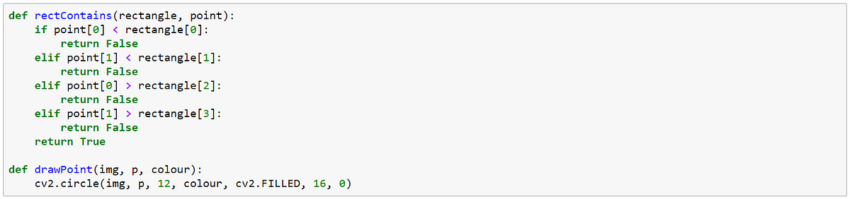
The helper function rectContains determines whether or not a point point falls within the image domain described by rectangle and thus whether or not it should be considered as input to the image’s Delaunay triangulation.
The drawPoint function does exactly that, i.e. it displays a facial landmark p in form of a coloured circle on the input image img.
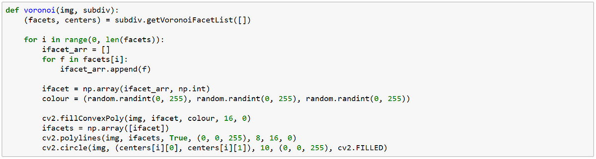
The voronoi function uses the subdiv member function getVoronoiFacetList to obtain and to subsequently draw the Voronoi diagram of an input image img based on its initial OpenCV subdivision subdiv. We set a random colour scheme for the Voronoi facet visualizations.
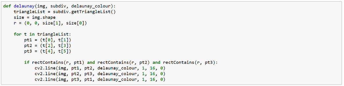
Similarly, the delaunay function determines and subsequently draws the triangles of the initial Delaunay subdivision subdiv of the input image img with the help of the subdiv member function getTriangleList.
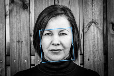
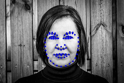
We apply these functions to the sample image shown in Figure 4. The facial bounding box and the corresponding facial landmarks were generated by the Face++ demo application.
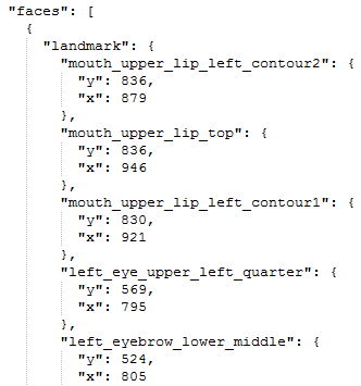
This demo service returns a JSON file which contains, amongst other things, the (x, y) coordinates of the facial landmarks detected by the service within the image domain. A JSON extract for the input image in Figure 4 is shown above.

These facial landmark coordinates represent the input points for the OpenCV subdivision function. We start the showcase generation by reading in the input image using the standard OpenCV imread method. The rectangular shape of the input image determines the subdivision domain stored in rect. The landmark points are uploaded in the form of “Face2Points.txt” into the points array. The subdivision itself is then instantiated and subsequently generated by inserting the facial landmark points one-by-one using the subdivision insert method.
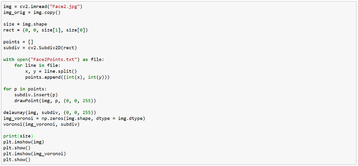
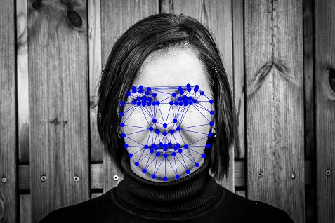
All that is then left to be done is to call our delaunay and voronoi functions passing on the input image and its newly generated subdivision. This results in the graphs displayed in Figure 5.
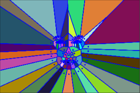
The animation in Figure 6 illustrates the Delaunay triangulation process of the input image one facial landmark point at a time.

The OpenCV subdiv object offers a variety of member functions for retrieving Delaunay or Voronoi edges and vertices. We refer to the OpenCV standard documentation for details. This way the various elements of these rather versatile geometric stuctures can easily be passed on to subsequent image processing or computer vision applications such as face segmentation, recognition [4, 5, 6] and morphing.
Although we focused on computer vision applications in this blog post, please note that there exist numerous use cases for these geometric structures, which extent well beyond the field of computer vision and include, in particular, other areas of applied AI such as robotic navigation. See, for example, [1,2] for inspiration.
References
[1] M. de Berg, O. Cheong, M. van Kreveld, and M. Overmars, Computational Geometry: Algorithms and Applications, 3rd edition, Springer, Berlin, Germany, 2010
[2] F. Aurenhammer, Voronoi Diagrams - A Survey of a Fundamental Geometric Data Structure, ACM Computing Surveys, 23(3), 1991, pp. 345–405
[3] R. Szeliski, Computer Vision: Algorithms and Applications, Springer, London, UK, 2011
[4] A. Cheddad, D. Mohamad, and A. A. Manaf, Exploiting Voronoi diagram properties in face segmentation and feature extraction, Pattern Recognition, Vol. 41, 2008, pp. 3842–3859
[5] M. A. Suhail, M. S. Obaidat, S. S. Ipson, and B. Sadoun, Content-based image segmentation, IEEE Int. Conf. Man Cybern. (SMC), Vol. 5, 2002
[6] M. Burge and W. Burger, Ear biometrics, in: A. Jain, R. Bolle, and S. Pankanti (eds.), Biometrics: Personal Identification in Networked Society, Kluwer Academic, Boston, MA, USA, 1999, pp. 273–285